5. Database services

5.1. Amazon RDS

Amazon Ralational Database Service (RDS) is a manageed relational database with a choice of 6 popular database engines: Amazon Aurora, MySQL, PostgreSQL, MariaDB, Microsoft SQL Server and Oracle. This service has the following characteristics:

• Easy to administer. As Amazon RDS is a managed service, you manage application optimization tasks (schema design, query construction, query optimization) and AWS manages infrastructure tasks (power, HVAC, network, rack & stack, installation, routine maintenance, automated patching, scaling and monitoring, industry compliance, isolation & security, backup & recovery, High Availability).
• Available and durable. It provides automatic Multi-AZ data replication, automated backup, snapshots, and failover.
• Highly scalable. It scales DB compute and storage with a few clicks with no application downtime.
• Fast and secure. It provides SSD storage and guaranteed provisioned I/O; data encryption at rest and in transit.

Amazon Relational Database Service (Amazon RDS)

5.1.1. Use cases

Amazon RDS is ideal for:

• Web and mobile applications that need a DB with high throughput, massive storage scalability, and HA. Since RDS does not have any licensing contraints, it perfectly fits the variable usage pattern of these applications.
• For E-commerce applications, RDS provides a flexible, secured, and low-cost DB solution for online sales and retailing.
• Mobile and online games require a DB platform with high throughput and HA. RDS manages the DB infrastructure so game developers don’t have to worry about provisioning, scaling or monitoring DB servers.

5.1.2. Get started with RDS

5.1.2.1. DB instances

The basic building block of Amazon RDS is the DB instance. A DB instance is an isolated DB environment that can contain multiple user-created DBs and can be accessed by using the same tools and applications that you use with an standalone DB instance. The resources found in a DB instance are determined by its DB instance class, and the type of storage is dictated by the type of disks. DB instances and storage differ in performance characteristics and price, allowing you to tailor your performance and cost to the needs of your DB. When you choose to create a DB instance, you first have to specify which DB engine to run. Amazon RDS currently supports 2 commercial engines (MS SQL Server and Oracle), 3 open source (MySQL, PostgreSQL, and MariaDB) and 1 cloud native (Amazon Aurora).

Amazon RDS DB instance

DB instances with commercial and open source DB engines use Amazon Elastic Block Store (Amazon EBS) volumes for database and log storage. Depending on the amount of storage requested, Amazon RDS automatically stripes across multiple Amazon EBS volumes to enhance performance. Amazon Aurora, which is MSQL and PostgreSQL compatible, uses purpose-built distributed, log-structured storage system.

If you are developing a new application, then it is recommended to go with the newest DB engine version. If you are migrating an existing application, then it is necessary to check compatibility requirements.

You can run Amazon RDS on VMware through the Amazon RDS connector. It packages technologies at the core of Amazon RDS in AWS and deploys them on premises. You need connectivity to AWS via a dedicated VPN tunnel enables database management entirely within your private data center.

You manage your DB engine configuration through the use of parameters in a DB parameter group. DB parameter groups act as a container for engine configuration values that are applied to one or more DB instances.

5.1.2.2. Instance types

Amazon RDS provides a selection of instance types optimized to fit different relational database use cases. Each instance type includes serveral instance sizes, allowing you to scale your database to the requirements of your target workload. Not every instance type is supported for every database engine, version, edition or region. The current Amazon RDS Instance Types are:

• General purpose: T3, T2, M5, M4.
• Memory optimized: R5, R4, X1e, X1, Z1d.

You can scale compute and memory vertically up or down. The new host is attaches to existing storage with minimal downtime. The endpoint will be the same, but you will have to reconnect to the new instance.

5.1.2.3. Storage types

Amazon RDS provides three storage types: General Purpose SSD (also known as gp2), Provisioned IOPS SSD (also known as io1), and magnetic. The following list briefly describes the three storage types:

• General Purpose SSD. General Purpose SSD volumes offer cost-effective storage that is ideal for a broad range of workloads. These volumes deliver single-digit millisecond latencies and the ability to burst to 3,000 IOPS for extended periods of time. Baseline performance for these volumes is determined by the volume’s size.
• Provisioned IOPS. Provisioned IOPS storage is designed to meet the needs of I/O-intensive workloads, particularly database workloads, that require low I/O latency and consistent I/O throughput.
• Magnetic. Amazon RDS also supports magnetic storage for backward compatibility. We recommend that you use General Purpose SSD or Provisioned IOPS for any new storage needs. The maximum amount of storage allowed for DB instances on magnetic storage is less than that of the other storage types.

General Purpose SSD is a great choice, but you have to be aware of burst credits on volumes less than 1 TB. Hitting credit-depletion results in IOPS drop, latencry and queue depth metrics will sppike until credits are replenished. You have to monitor BurstBalance to see the percent of burst-bucket I/O credits available. You have to monitor read/write IOPS to see if average IOPS is greater than the baseline. You can think General Purpose SSD burst rate and PIOPS stated rate as maximum I/O rates.

You can scale up Amazon EBS storage with no downtime. Initial scaling operation may take longer, because storage is reconfigured on older instances. You can re-provision IOPS on the fly without any disruption in the storage. You are limited to scale up to once every 6 hours.

5.1.3. Managing High Availability, read replicas, and backups

5.1.3.1. High Availability with Multi-AZ

Multi-AZ provides enterprise-grade fault-tolerance solution for production databases. Once configured, Amazon RDS automatically generates a standby copy of the primary instance in another AZ within the same Amazon VPC. Each DB instance manages a set of Amazon EBS volumes with a full copy of the data. After seeding the DB copy, transactions are synchronously replicated to the standby copy. Instances are monitored by an external observer to maintain consensus over quorum.

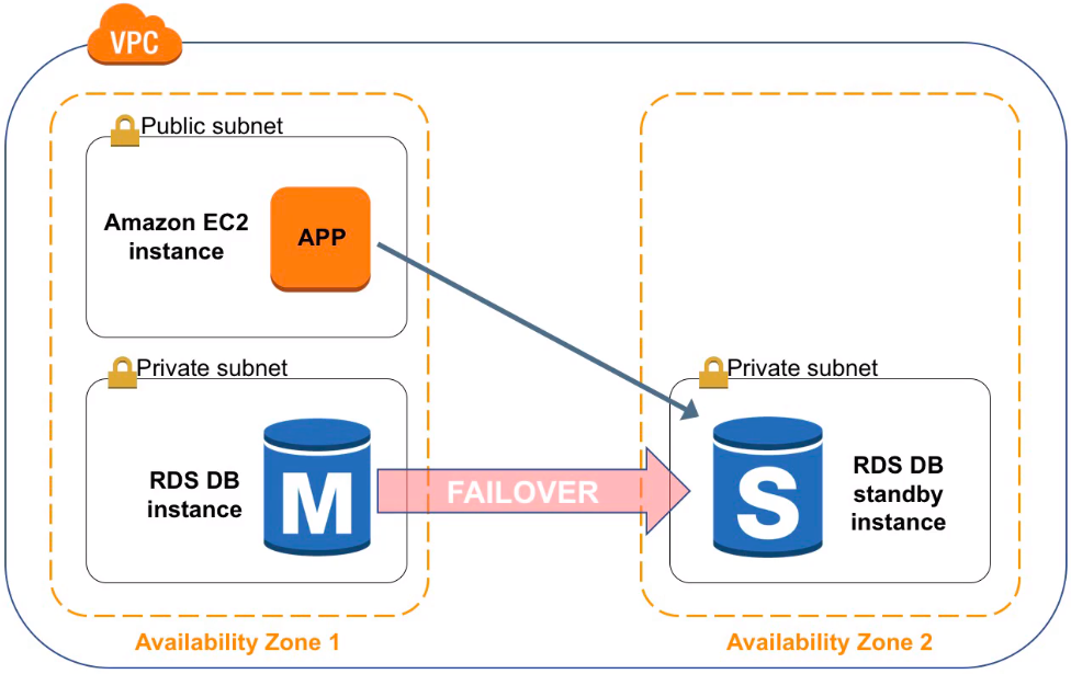
High Availability with Multi-AZ

In Amazon RDS, failover is automatically handled so that you can resume database operations as quickly as possible without administrative intervention in the event that your primary database instance went down. When failing over, Amazon RDS simply flips the canonical name record (CNAME) for your DB instance to point at the standby, which is in turn promoted to become the new primary.

Running a DB instance with Multi-AZ can enhance availability during planned system maintenance and help protect your DBs against DB instance failure and AZ disruption. If the master DB instance fails, Amazon RDS automatically brings the standby DB online as the new primary. Failover can be initiated by automation or through the Amazon RDS API. Because of the synchronous replication, there should be no data loss. As your applications reference the DB by name using RDS DNS endpoint, you don’t need to change anything in your application code to use the standby copy for failover. A new DB instance in the AZ where it was located the failed previous primary DB instance is provisioned as the new secondary DB instance.

Amazon RDS automatically performs a failover in the event of any of the following:

• Loss of availability in primary Availability Zone.
• Loss of network connectivity to primary.
• Compute unit failure on primary.
• Storage failure on primary.

Note

It is important to have in mind that it detects infrastructure issues, not database engine problems.

Important

The standby instance will not perform any read and write operations while the primary instance is running.

In case of a Single-AZ database failure, a user-initiated point-in-time-restore operation will be required. This operation can take several hours to complete, and any data updates that occurred after the latest restorable time (typically within the last five minutes) will not be available.

5.1.3.2. Read scalability with Amazon RDS Read Replicas

Amazon RDS can gain read scalability with the creation of read replicas for MySQL, MariaDB, and PostgreSQL. Updates made to the source DB instance are asynchronously copied to the read replica instance. You can reduce the load on your source DB instance by routing read queries from your applications to the read replica. Using read replicas, you can also scale out beyond the capacity constraints of a single DB instance for read-heavy DB workloads. It brings data close to your applications in different regions.

Amazon RDS read replicas

You can create up to 5 replicas per source database. You can monitor replication lag in Amazon CloudWatch or Amazon RDS console. Read replicas can be created in a different region than the master DB. This feature can help satisfy DR requirements or cutting down on latency by directing reads to a read replica closer to the user. Single-region read replicas is supported for Oracle EE and is coming soon for SQL Server.

Read replicas can also be promoted to become the master DB instance, but due to the asynchronous replication, this requires manual action. You can do it for faster recovery in the event of a disaster. You can upgrade a read replica to a new engine version.

Amazon RDS Read Replicas provide enhanced performance and durability for database (DB) instances. This feature makes it easy to elastically scale out beyond the capacity constraints of a single DB instance for read-heavy database workloads. You can create one or more replicas of a given source DB Instance and serve high-volume application read traffic from multiple copies of your data, thereby increasing aggregate read throughput.

Multi-AZ vs Read Replicas

Multi-AZ	Read Replicas
Synchronous replication: highly durable	Asynchronous replication: highly scalable
Only primary instance is active at any point in time	All replicas are active and can be used for read scaling
Backups can be taken from secondary	No backups configured by default
Always in 2 AZs within a region	It can be within an AZ, cross-AZ, or cross-region
Database engine version upgrades happen on primary	Database engine version upgrades independently from source instance
Automatic failover when a problem is detected	It can be manually promoted to a standalone database

How do I make my RDS MySQL read replica writable?

5.1.3.3. Plan for DR

You can plan for disaster recovery by using automated backups and manual snapshots. You can use a cross-region read replica as a standby database for recovery in the event of a disaster. Read replicas can be configured for Multi-AZ to reduce recovery time.

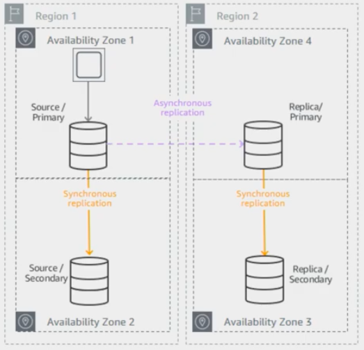
Disaster recovery with Multi-AZ and read replicas

This architecture is supported for MySQL, MariaDB and PostgreSQL. For Oracle and SQL Server, you can use cross-region backup copies.

Note

You can use delayed replication for MySQL to protect from self-inflicted disasters.

5.1.3.4. Backups

Amazon RDS can manage backups using one of these two options:

• You can do manual snapshots. These are storage level snapshots with no performance penalty for backups in multi-AZ configurations and only a brief pause in you I/O for single-AZ configurations. It leverages EBS snapshots stored in Amazon S3.
• Automated backups gives you a point-in-time restore capability. AWS will take snapshots once a day and capture transactions logs and store them every 5 minutes in S3.

Snapshots can be copied across regions or shared with other accounts.

Automated backups vs Manual snapshots

Automated backups	Manual snapshots
Specify backup retention window per instance (7-day default)	Manually created through AWS console, AWS CLI, or Amazon RDS
Kept unitl outside of window (35-day maximum) or instance is deleted	Kept until you delete them
Supports PITR	Restores to saved snapshot
Good for DR	Use for checkpoint before making large changes, non-production/test environments, final copy before deleting a database

When you restore a backup, you are creating a entirely new DB instance. In this process, it is defined the instance configuration just like a new instance. It will get the default parameters, security, and option groups.

Restoration can get a long period of time because new volumes are hydrated from Amazon S3. While the volume is usable immediately, full performance requires the volume to be initialized until fully instantiated. One way to mitigate the length of the restoration process is to migrate to a DB instance class with high I/O capacity and later downsizes it. You should maximize I/O during restore process.

5.1.4. Security controls

Amazon RDS is designed to be secure by default. Network isolation is provided with Amazon VPC. AWS IAM based resource-level permission controls are supported. It provides encryption at rest using AWS KMS (for all engines) or Oracle/Microsoft Transparent Data Encryption (TDE). SSL protection for data in transit is used.

5.1.4.1. Identity and Access Management

You can use IAM to control who can perform actions on RDS resources. It is recommended not to use AWS root credentials to manage Amazon RDS resources, you should create an IAM user for everyone, including the administrator. You can use AWS MFA to provide extra level of protection.

5.1.4.1.1. IAM Database Authentication for MySQL and PostgreSQL

You can authenticate to your DB instance using AWS Identity and Access Management (IAM) database authentication. IAM database authentication works with MySQL and PostgreSQL. With this authentication method, you don’t need to use a password when you connect to a DB instance. Instead, you use an authentication token.

An authentication token is a unique string of characters that Amazon RDS generates on request. Authentication tokens are generated using AWS Signature Version 4. Each token has a lifetime of 15 minutes. You don’t need to store user credentials in the database, because authentication is managed externally using IAM. You can also still use standard database authentication.

Database options

For enabling RDS IAM authentication, you should check the “Enable IAM DB authentication” option on RDS modify or create phase.

Database authentication

After this step, you should create a user for your database account and use “FLUSH PRIVILEGES;“ command in MySQL. The DB user account has to use same name with your IAM account.

Create user phase for MySQL

mysql > CREATE USER myuser IDENTIFIED WITH AWSAuthenticationPlugin AS 'RDS';
Query OK, 0 rows affected (0.18 sec)

Create user phase for PostgreSQL

# psql --host postgres-sample-instance.cbr4qtvbvyrz.us-east-2.rds.amazonaws.com --username-postgres
Password for user postgres:
psql (9.5.19, server 11.5)
SSL connection (protocol: TLSv1.2, cipher: ECDHE-RSA-AES256-GCM-SHA384, bits: 256, compression: off)
Type "help" for help.

postgres-> CREATE USER myuser WITH LOGIN;
CREATE ROLE
postgres-> GRANT rds_iam TO myuser;
GRANT ROLE

After this command, you have to add an IAM role to your IAM user for creating a relation between your IAM account and RDS DB user.

IAM database authentication provides the following benefits:

1. Network traffic to and from the database is encrypted using Secure Sockets Layer (SSL).
2. You can use IAM to centrally manage access to your database resources, instead of managing access individually on each DB instance.
3. For applications running on Amazon EC2, you can use profile credentials specific to your EC2 instance to access your database instead of a password, for greater security

How To Connect an AWS RDS Instance with IAM User Authentication

5.1.5. Encryption

You can use AWS KMS-based encryption in the AWS console. There is no performance penalty for encrypting data and it is performed at the volume level. It provides you with a centralized access and audit of key activity. It uses two-tier encryption with the customer master key provided by you and each individual instance has its data key, which is used to encrypt the data.

Database encryption

Best practices for encryption are follow with RDS:

• Encryption cannot be removed from DB instances.
• If source is encrypted, Read Replicas must be encrypted.
• Add encryption to an uncrypted DB instance by encrypting a snapshot copy.

5.1.5.1. Microsoft SQL Server

You can use Secure Sockets Layer (SSL) to encrypt connections between your client applications and your Amazon RDS DB instances running Microsoft SQL Server. SSL support is available in all AWS regions for all supported SQL Server editions.

When you create a SQL Server DB instance, Amazon RDS creates an SSL certificate for it. The SSL certificate includes the DB instance endpoint as the Common Name (CN) for the SSL certificate to guard against spoofing attacks. There are 2 ways to use SSL to connect to your SQL Server DB instance:

• Force SSL for all connections, this happens transparently to the client, and the client doesn’t have to do any work to use SSL.
• Encrypt specific connections, this sets up an SSL connection from a specific client computer, and you must do work on the client to encrypt connections.

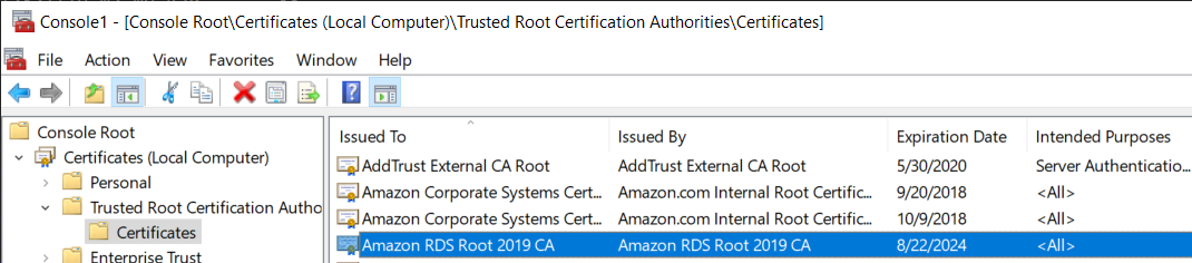
SSL certificate

You can force all connections to your DB instance to use SSL, or you can encrypt connections from specific client computers only. To use SSL from a specific client, you must obtain certificates for the client computer, import certificates on the client computer, and then encrypt the connections from the client computer.

If you want to force SSL, use the rds.force_ssl parameter. By default, the rds.force_ssl parameter is set to false. Set the rds.force_ssl parameter to true to force connections to use SSL. The rds.force_ssl parameter is static, so after you change the value, you must reboot your DB instance for the change to take effect.

5.1.6. Monitoring

5.1.6.1. Monitor

Amazon RDS comes with comprehensive monitoring built-in:

• Amazon CloudWatch metrics and alarms. It allows you to monitor core metrics:

  • CPU/Storage/Memory
  • Swap usage
  • I/O (read and write)
  • Latency (read and write)
  • Throughput (read and write)
  • Replica lag

The monitoring interval is usually down to 1 minute. You can configure alarms on these metrics.

• Amazon CloudWatch logs. It allows publishing DB logs (errors, audit, slow queries) to a centralized log store (except SQL Server). You can access logs directly from RDS console and API for all engines.
• Enhanced monitoring. It is an agent-based monitoring system that allows you to have access to over 50 CPU, memory, file system, database engine, and disk I/O metrics. It is configurable to monitor up to 1 second intervals. They are automatically published to Amazon CloudWatch logs on your behalf.

Amazon RDS provides metrics in real time for the operating system (OS) that your DB instance runs on. You can view the metrics for your DB instance using the console, or consume the Enhanced Monitoring JSON output from CloudWatch Logs in a monitoring system of your choice. By default, Enhanced Monitoring metrics are stored in the CloudWatch Logs for 30 days. To modify the amount of time the metrics are stored in the CloudWatch Logs, change the retention for the RDSOSMetrics log group in the CloudWatch console.

Take note that there are certain differences between CloudWatch and Enhanced Monitoring Metrics. CloudWatch gathers metrics about CPU utilization from the hypervisor for a DB instance, and Enhanced Monitoring gathers its metrics from an agent on the instance. As a result, you might find differences between the measurements, because the hypervisor layer performs a small amount of work.

The differences can be greater if your DB instances use smaller instance classes, because then there are likely more virtual machines (VMs) that are managed by the hypervisor layer on a single physical instance. Enhanced Monitoring metrics are useful when you want to see how different processes or threads on a DB instance use the CPU and memory.

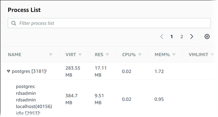
Use of CPU and memory of processes or threads on a DB instance

In RDS, the Enhanced Monitoring metrics shown in the Process List view are organized as follows:

• RDS child processes. Shows a summary of the RDS processes that support the DB instance, for example aurora for Amazon Aurora DB clusters and mysqld for MySQL DB instances. Process threads appear nested beneath the parent process. Process threads show CPU utilization only as other metrics are the same for all threads for the process. The console displays a maximum of 100 processes and threads. The results are a combination of the top CPU consuming and memory consuming processes and threads. If there are more than 50 processes and more than 50 threads, the console displays the top 50 consumers in each category. This display helps you identify which processes are having the greatest impact on performance.
• RDS processes. Shows a summary of the resources used by the RDS management agent, diagnostics monitoring processes, and other AWS processes that are required to support RDS DB instances.
• OS processes. Shows a summary of the kernel and system processes, which generally have minimal impact on performance.

• Performance Insights uses lightweight data collection methods that don’t impact the performance of your applications, and makes it easy to see which SQL statements are causing the load, and why. It requires no configuration or maintenance, and is currently available for Amazon Aurora (PostgreSQL- and MySQL-compatible editions), Amazon RDS for PostgreSQL, MySQL, MariaDB, SQL Server and Oracle. It provides an easy and powerful dashboard showing load on your database. It helps you identify source of bottlenecks: top SQL queries, wait statistics. It has an adjustable time frame (hour, day week, month). With 7 days of free performance history retention, it’s easy to track down and solve a wide variety of issues. If you need longer-term retention, you can choose to pay for up to two years of performance history retention.

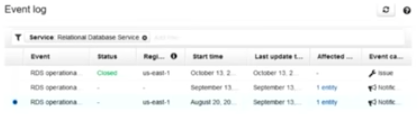
5.1.6.2. Events

Amazon RDS event notifications let you know when important things happen. You can leverage built-in notifications via Amazon SNS. Events are published to Amazon CloudWatch Events, where you can create rules to respond to the events. It supports cross-account event delivery. There are 6 different source types: DB instance, DB parameter group, DB security group, DB snapshot, DB cluster, DB cluster snapshot. There are 17 different event categories, such as availability, backup, deletion, configuration change, etc.

5.1.7. Maintenance and billing

5.1.7.1. Maintenance

Any maintenance that causes downtime (typically only a few times per year) will be scheduled in your maintenace window. Operating system or Amazon RDS software patches are usually performed without restarting databases. Database engine upgrades require downtime:

• Minor version upgrades: automatic or manually applied.
• Major version upgrades: manually applied because there can be application compatibility issues.
• Version deprecation: 3-6-month notification before scheduled upgrades.

You an view upcoming maintenance events in your AWS Personal Health Dashboard.

AWS Personal Health Dashboard

5.1.7.2. Billing

To estimate the cost of using RDS, you need to consider the following factors:

• Database instance (instance hours), from the time you launch a DB instance until you terminate it. It depends on Database characteristics: a combination of region, instance type, DB engine, and license (optional).
• Database storage (GB-mo). It can be either provisioned (Amazon EBS) or consumed (Amazon Aurora). If you are using provisioned IOPS for io1 storage type in IOPS-Mo. You are charged for the number of database input and output requests for Amazon Aurora and Amazon EBS magnetic-storage types. If your purchase options is on-demand DB, then instances are charged by the hour. Reserved DB instances require upfront payment for DB instances reserved.
• Backup storage (GB-mo). Size of backups and snapshots stored in Amazon S3. There is no additional charge for backup storage of up to 100% of your provisioned DB storage for an active DB instance. After the DB instance is terminated, backup storage is billed per GB/month.
• Number of database instances, to handle peak loads.
• Deployment type. You can deploy the DB to a single AZ or multiple AZs.
• Outbound data transfer is tiered and inbound data transfer is free.

In order to reduce costs you can stop and start a DB instance from the console, AWS CLIs and SDKs. You can stop and start a DB instance whether it is configured for a single Availability Zone or for Multi-AZ, for database engines that support Multi-AZ deployments. You can’t stop an Amazon RDS for SQL Server DB instance in a Multi-AZ configuration.

When you stop a DB instance, the DB instance performs a normal shutdown and stops running. The status of the DB instance changes to stopping and then stopped. Any storage volumes remain attached to the DB instance, and their data is kept. Any data stored in the RAM of the DB instance is deleted.

Stopping a DB instance removes pending actions, except for pending actions for the DB instance’s option group or DB parameter group. While DB instance is stopped, you only pay for storage. The backup retention window is maintained while stopped.

Important

You can stop a DB instance for up to 7 days. If you don’t manually start your DB instance after 7 days, your DB instance is automatically started so that it doesn’t fall behind any required maintenance updates. You cannot stop DB instances that have read replicas or are read replicas. If you want to stop a DB instance for more than 7 days, a possible strategy is to take an snasphot.

You can also save money by using Reverved Instances (RIs) that provide a discount over on-demand prices. You have to match region, instance family and engine of on-demand usage to apply benefit. There is size flexibility available for open source and Oracle BYOL engines. By default, RIs are shared among all accounts in consolidated billing. You can use the RI utilization and coverage reports to determine how your RIs are being used. Amazon RDS RI recommendations report uses historical data to recommend which RIs to buy.

5.1.8. Best practices

5.1.8.1. MySQL

• Ensure that automated backups are enabled for the RDS.
• Use InnoDB as the storage engine for MySQL.
• Partition your large tables so that file sizes does not exceed the 16 TB limit.

5.2. Amazon Aurora

5.2.1. Introduction

Amazon Aurora is a fully managed, relational DBaaS that combines the speed and reliability of high-end commercial DBs, with the simplicity and cost-effectiveness of open source databases. It is designed to be compatible with MySQL and PostgreSQL, so existing applications and tools, can run against it without modification. It follows a simple pay as you go pricing model.

It is part of Amazon RDS and it tightly integrated with an SSD-backend virtualized storage layer purposefully built to accelerate DB workloads. It delivers up to 5 times the throughput of standard MySQL and up to 3 times the throughput of standard PostgreSQL.

It can scale automatically an non-disruptively, expanding up to 64 TB and rebalancing storage I/O to provide consistent performance, without the need for over-provisioning. Aurora storage is also fault-tolerant and self-healing, so any storage failures are repaired transparently.

It automatically replicates your storage six ways, across three Availability Zones. Amazon Aurora storage is fault-tolerant, transparently handling the loss of up to two copies of data without affecting database write availability and up to three copies without affecting read availability. Aurora always replicates your data across three Availability Zones, regardless of whether your database uses read replicas.

It is a regional service that offers greater than 99.99% availability. The service is designed to automatically detect DB crashes and restart the DB without the need for crash recovery or DB rebuilds. If the entire instance fails, Amazon Aurora automatically fails over to one of up to 15 read replicas.

AWS re:Invent 2018: [REPEAT 1] Deep Dive on Amazon Aurora with MySQL Compatibility (DAT304-R1)

5.2.2. Performance

Aurora scale out, distributed architecture made two main contributions:

1. Push log applicator to storage. That allows us to construct pages from the logs themselves. It is not necessary to write full pages anymore. Unlike traditional databases that have to write logs and pages, Aurora only writes logs. This means that there is significantly less I/O and warm up. There is no checkpointing, you don’t have to worry about cache additions,…
2. Instead of using heavy consistency protocols, Aurora uses 4/6 write quorum with local tracking.

The benefits of this are:

• Better write performance.
• Read scale out because the replicas are sharing the storage with the master.
• AZ+1 failure tolerance. Aurora stores 6 copies: 2 copies per AZ.
• Instant database redo recovery, even if an entire AZ goes down.

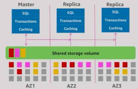
Aurora architecture

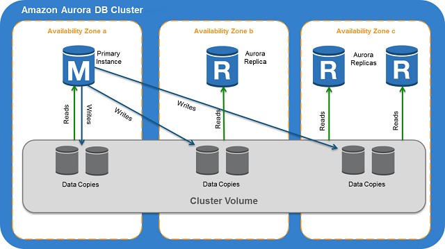
Amazon Aurora typically involves a cluster of DB instances instead of a single instance. Each connection is handled by a specific DB instance. When you connect to an Aurora cluster, the host name and port that you specify point to an intermediate handler called an endpoint. Aurora uses the endpoint mechanism to abstract these connections. Thus, you don’t have to hardcode all the hostnames or write your own logic for load-balancing and rerouting connections when some DB instances aren’t available.

For certain Aurora tasks, different instances or groups of instances perform different roles. For example, the primary instance handles all data definition language (DDL) and data manipulation language (DML) statements. Up to 15 Aurora Replicas handle read-only query traffic.

Using endpoints, you can map each connection to the appropriate instance or group of instances based on your use case. For example, to perform DDL statements you can connect to whichever instance is the primary instance. To perform queries, you can connect to the reader endpoint, with Aurora automatically performing load-balancing among all the Aurora Replicas. For clusters with DB instances of different capacities or configurations, you can connect to custom endpoints associated with different subsets of DB instances. For diagnosis or tuning, you can connect to a specific instance endpoint to examine details about a specific DB instance.

The custom endpoint provides load-balanced database connections based on criteria other than the read-only or read-write capability of the DB instances. For example, you might define a custom endpoint to connect to instances that use a particular AWS instance class or a particular DB parameter group. Then you might tell particular groups of users about this custom endpoint. For example, you might direct internal users to low-capacity instances for report generation or ad hoc (one-time) querying, and direct production traffic to high-capacity instances.

5.2.3. Amazon Aurora Replicas

Amazon Aurora MySQL and Amazon Aurora PostgreSQL support Amazon Aurora Replicas, which share the same underlying volume as the primary instance. Updates made by the primary are visible to all Amazon Aurora Replicas. With Amazon Aurora MySQL, you can also create MySQL Read Replicas based on MySQL’s binlog-based replication engine. In MySQL Read Replicas, data from your primary instance is replayed on your replica as transactions. For most use cases, including read scaling and high availability, it is recommended using Amazon Aurora Replicas.

Aurora failover

Read Replicas are primarily used for improving the read performance of the application. The most suitable solution in this scenario is to use Multi-AZ deployments instead but since this option is not available, you can still set up Read Replicas which you can promote as your primary stand-alone DB cluster in the event of an outage.

5.2.4. Failover

Failover is automatically handled by Amazon Aurora so that your applications can resume database operations as quickly as possible without manual administrative intervention.

If you have an Amazon Aurora Replica in the same or a different Availability Zone, when failing over, Amazon Aurora flips the canonical name record (CNAME) for your DB Instance to point at the healthy replica, which in turn is promoted to become the new primary. Start-to-finish, failover typically completes within 30 seconds.

If you are running Aurora Serverless and the DB instance or AZ become unavailable, Aurora will automatically recreate the DB instance in a different AZ.

If you do not have an Amazon Aurora Replica (i.e. single instance) and are not running Aurora Serverless, Aurora will attempt to create a new DB Instance in the same Availability Zone as the original instance. This replacement of the original instance is done on a best-effort basis and may not succeed, for example, if there is an issue that is broadly affecting the Availability Zone.

You can use the reader endpoint to provide high availability for your read-only queries from your DB cluster by placing multiple Aurora Replicas in different Availability Zones and then connecting to the read-only endpoint for your read workload. The reader endpoint also load-balances connections to the Aurora Replicas in a DB cluster.

5.3. Amazon DynamoDB

5.3.1. Introduction

Amazon DynamoDB is a fast and flexible NoSQL database service for all applications that need consistent, single-digit millisecond latency at any scale. It is a fully managed cloud database and supports both document and key-value store models. Its flexible data model, reliable performance, and automatic scaling of throughput capacity makes it a great fit for mobile, web, gaming, ad tech, IoT, and many other applications. It is fast and consistent because it has a fully distributed request router. It provides fine-grained access control for accessing, for instance: the tables, the attributes within an item, etc. It allows event driven programming.

SQL vs NoSQL

SQL	NoSQL
Optimized for storage	Optimized for compute
Normalized/relational	Denormalized/hierarchical
Ad hoc queries	Instantiated views
Scale vertically	Scale horizontally
Good for OLAP	Built for OLTP at scale

The following are the basic DynamoDB components:

• Tables. Similar to other database systems, DynamoDB stores data in tables. A table is a collection of data. For example, see the example table called People that you could use to store personal contact information about friends, family, or anyone else of interest. You could also have a Cars table to store information about vehicles that people drive.
• Items. Each table contains zero or more items. An item is a group of attributes that is uniquely identifiable among all of the other items. In a People table, each item represents a person. For a Cars table, each item represents one vehicle. Items in DynamoDB are similar in many ways to rows, records, or tuples in other database systems. In DynamoDB, there is no limit to the number of items you can store in a table.
• Attributes. Each item is composed of one or more attributes. An attribute is a fundamental data element, something that does not need to be broken down any further. For example, an item in a People table contains attributes called PersonID, LastName, FirstName, and so on. For a Department table, an item might have attributes such as DepartmentID, Name, Manager, and so on. Attributes in DynamoDB are similar in many ways to fields or columns in other database systems.

When you create a table, in addition to the table name, you must specify the primary key of the table. The primary key uniquely identifies each item in the table, so that no two items can have the same key.

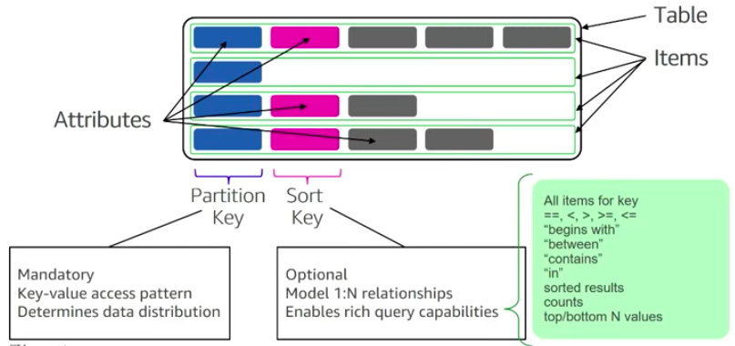
DynamoDB tables, items and attributes

DynamoDB supports two different kinds of primary keys:

• Partition key A simple primary key, composed of one attribute known as the partition key. DynamoDB uses the partition key’s value as input to an internal hash function. The output from the hash function determines the partition (physical storage internal to DynamoDB) in which the item will be stored. In a table that has only a partition key, no two items can have the same partition key value. It allows table to be partitioned for scale.

Partition keys

• Partition key and sort key. Referred to as a composite primary key, this type of key is composed of two attributes. The first attribute is the partition key, and the second attribute is the sort key. All items with the same partition key value are stored together, in sorted order by sort key value. In a table that has a partition key and a sort key, it’s possible for two items to have the same partition key value. However, those two items must have different sort key values. There is no limit on the number of items per partition key, except if you have local secondary indexes.

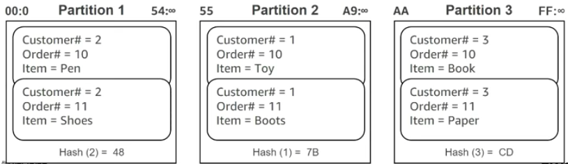
Partition: Sort key

Partitions are three-way replicated. In DynamoDB, you get an acknowledge when two of these replicas has been done.

The partition key portion of a table’s primary key determines the logical partitions in which a table’s data is stored. This in turn affects the underlying physical partitions. Provisioned I/O capacity for the table is divided evenly among these physical partitions. Therefore a partition key design that doesn’t distribute I/O requests evenly can create “hot” partitions that result in throttling and use your provisioned I/O capacity inefficiently.

The optimal usage of a table’s provisioned throughput depends not only on the workload patterns of individual items, but also on the partition-key design. This doesn’t mean that you must access all partition key values to achieve an efficient throughput level, or even that the percentage of accessed partition key values must be high. It does mean that the more distinct partition key values that your workload accesses, the more those requests will be spread across the partitioned space. In general, you will use your provisioned throughput more efficiently as the ratio of partition key values accessed to the total number of partition key values increases.

One example for this is the use of partition keys with high-cardinality attributes, which have a large number of distinct values for each item.

DynamoDB supports in-place atomic updates. It supports both increment and decrement atomic operations.

AWS re:Invent 2018: Amazon DynamoDB Deep Dive: Advanced Design Patterns for DynamoDB (DAT401)

5.3.2. DynamoDB Streams

A DynamoDB stream is an ordered flow of information about changes to items in an Amazon DynamoDB table. When you enable a stream on a table, DynamoDB captures information about every modification to data items in the table.

Whenever an application creates, updates, or deletes items in the table, DynamoDB Streams writes a stream record with the primary key attribute(s) of the items that were modified. A stream record contains information about a data modification to a single item in a DynamoDB table. You can configure the stream so that the stream records capture additional information, such as the “before” and “after” images of modified items.

Amazon DynamoDB is integrated with AWS Lambda so that you can create triggers—pieces of code that automatically respond to events in DynamoDB Streams. With triggers, you can build applications that react to data modifications in DynamoDB tables.

If you enable DynamoDB Streams on a table, you can associate the stream ARN with a Lambda function that you write. Immediately after an item in the table is modified, a new record appears in the table’s stream. AWS Lambda polls the stream and invokes your Lambda function synchronously when it detects new stream records.

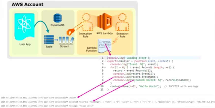
DynamoDB Streams and AWS Lambda

You can create a Lambda function which can perform a specific action that you specify, such as sending a notification or initiating a workflow. For instance, you can set up a Lambda function to simply copy each stream record to persistent storage, such as EFS or S3, to create a permanent audit trail of write activity in your table.

5.3.3. DynamoDB auto scaling

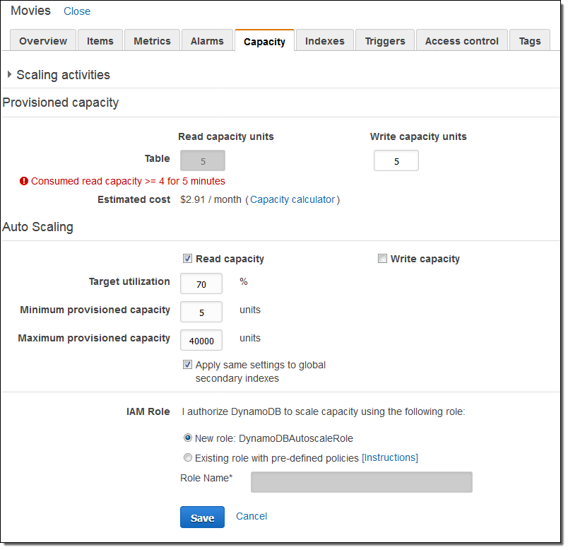
DynamoDB auto scaling uses the AWS Application Auto Scaling service to dynamically adjust provisioned throughput capacity on your behalf, in response to actual traffic patterns. This enables a table or a global secondary index to increase its provisioned read and write capacity to handle sudden increases in traffic, without throttling. When the workload decreases, Application Auto Scaling decreases the throughput so that you don’t pay for unused provisioned capacity.

5.3.4. Use cases

• Managing web sessions. DynamoDB Time-to-Live (TTL) mechanism enables you to manage web sessions of your application easily. It lets you set a specific timestamp to delete expired items from your tables. Once the timestamp expires, the corresponding item is marked as expired and is subsequently deleted from the table. By using this functionality, you do not have to track expired data and delete it manually. TTL can help you reduce storage usage and reduce the cost of storing data that is no longer relevant.
• Storing metadata for Amazon S3 objects. Amazon DynamoDB stores structured data indexed by primary key and allow low latency read and write access to items ranging from 1 byte up to 400KB. Amazon S3 stores unstructured blobs and is suited for storing large objects up to 5 TB. In order to optimize your costs across AWS services, large objects or infrequently accessed data sets should be stored in Amazon S3, while smaller data elements or file pointers (possibly to Amazon S3 objects) are best saved in Amazon DynamoDB.

To speed up access to relevant data, you can pair Amazon S3 with a search engine such as Amazon CloudSearch or a database such as Amazon DynamoDB or Amazon RDS. In these scenarios, Amazon S3 stores the actual information, and the search engine or database serves as the repository for associated metadata such as the object name, size, keywords, and so on. Metadata in the database can easily be indexed and queried, making it very efficient to locate an object’s reference by using a search engine or a database query. This result can be used to pinpoint and retrieve the object itself from Amazon S3.

5.3.5. Amazon DynamoDB Accelerator (DAX)

Amazon DynamoDB Accelerator (DAX) is a fully managed, highly available, in-memory cache for DynamoDB that delivers up to a 10x performance improvement ? from milliseconds to microseconds ? even at millions of requests per second. DAX does all the heavy lifting required to add in-memory acceleration to your DynamoDB tables, without requiring developers to manage cache invalidation, data population, or cluster management.

Amazon DynamoDB Accelerator (DAX) configuration

DAX is a DynamoDB-compatible caching service that enables you to benefit from fast in-memory performance for demanding applications. DAX addresses three core scenarios:

1. As an in-memory cache, DAX reduces the response times of eventually consistent read workloads by an order of magnitude, from single-digit milliseconds to microseconds.
2. DAX reduces operational and application complexity by providing a managed service that is API-compatible with DynamoDB. Therefore, it requires only minimal functional changes to use with an existing application.
3. For read-heavy or bursty workloads, DAX provides increased throughput and potential operational cost savings by reducing the need to overprovision read capacity units. This is especially beneficial for applications that require repeated reads for individual keys.

DAX supports server-side encryption. With encryption at rest, the data persisted by DAX on disk will be encrypted. DAX writes data to disk as part of propagating changes from the primary node to read replicas. The following diagram shows a high-level overview of DAX.

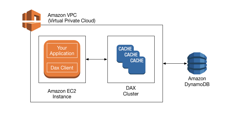
High-level overview of DAX

5.4. Amazon Redshift

5.4.1. Architecture and concepts

Amazon Redshift is a fast, scalable data warehouse that makes it simple and cost-effective to analyze all your data across your data warehouse and data lake. Redshift delivers ten times faster performance than other data warehouses by using machine learning, massively parallel query execution, and columnar storage on high-performance disk. Redshift is a fully-managed service which is the result of rewriting PostgreSQL to:

• Become a columnar database.
• Provide MPP (massive parallel processing) that allows to scale out up to a several petabytes database.
• Provide analytics functions to work as an OLAP service.

It is also integrated with the rest of the AWS ecosystem: S3, KMS, Route 53, etc.

The maintenance window occurs weekly, and DB instances can receive upgrades to the operating system (OS) or to the DB engine. AWS requires at least a 30-minute window in your instance’s weekly schedule to confirm that all instances have the latest patches and upgrades. During the maintenance window, tasks are performed on clusters and instances. For the security and stability of your data, maintenance can cause instances to be unavailable.

The maintenance window defines when the deployment or operation begins, but maintenance itself can take longer to complete. As a result, the time used for some operations can exceed the duration of the maintenance window.

5.4.1.1. Architecture

The elements of the Amazon Redshift data warehouse architecture is shown in the following figure.

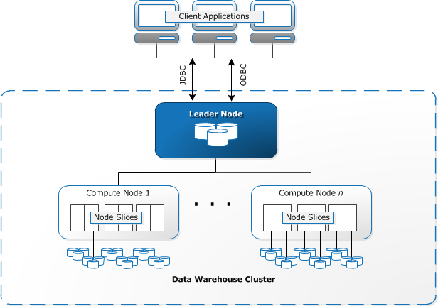
Amazon Redshift architecture

5.4.1.1.1. Client applications

Amazon Redshift integrates with various data loading and ETL (extract, transform, and load) tools and business intelligence (BI) reporting, data mining, and analytics tools. Amazon Redshift is based on industry-standard PostgreSQL, so most existing SQL client applications will work with only minimal changes. Amazon Redshift communicates with client applications by using industry-standard JDBC and ODBC drivers for PostgreSQL.

5.4.1.1.2. Leader node

The leader node manages communications with client programs and all communication with compute nodes. It parses and develops execution plans to carry out database operations, in particular, the series of steps necessary to obtain results for complex queries. Based on the execution plan, the leader node compiles code, distributes the compiled code to the compute nodes, and assigns a portion of the data to each compute node.

The leader node distributes SQL statements to the compute nodes only when a query references tables that are stored on the compute nodes. All other queries run exclusively on the leader node. Amazon Redshift is designed to implement certain SQL functions only on the leader node. A query that uses any of these functions will return an error if it references tables that reside on the compute nodes.

5.4.1.1.3. Clusters

The core infrastructure component of an Amazon Redshift data warehouse is a cluster. A cluster is composed of one or more compute nodes. If a cluster is provisioned with two or more compute nodes, an additional leader node coordinates the compute nodes and handles external communication. Your client application interacts directly only with the leader node. The compute nodes are transparent to external applications.

5.4.1.1.4. Compute nodes

The leader node compiles code for individual elements of the execution plan and assigns the code to individual compute nodes. The compute nodes execute the compiled code and send intermediate results back to the leader node for final aggregation.

Each compute node has its own dedicated CPU, memory, and attached disk storage, which are determined by the node type. As your workload grows, you can increase the compute capacity and storage capacity of a cluster by increasing the number of nodes, upgrading the node type, or both.

Amazon Redshift provides two node types; dense storage nodes and dense compute nodes. Each node provides two storage choices. You can start with a single 160 GB node and scale up to multiple 16 TB nodes to support a petabyte of data or more.

Hopefully all the data is spread across the compute nodes. The SQL queries are executed in parallel and that’s why it is called a massively parallel, shared nothing columnar architecture.

5.4.1.1.5. Node slices

A compute node is partitioned into slices. Each slice is allocated a portion of the node’s memory and disk space, where it processes a portion of the workload assigned to the node. The leader node manages distributing data to the slices and apportions the workload for any queries or other database operations to the slices. The slices then work in parallel to complete the operation. The number of slices per node is determined by the node size of the cluster.

When you create a table, you can optionally specify one column as the distribution key. When the table is loaded with data, the rows are distributed to the node slices according to the distribution key that is defined for a table. Choosing a good distribution key enables Amazon Redshift to use parallel processing to load data and execute queries efficiently.

5.4.1.1.6. Internal network

Amazon Redshift takes advantage of high-bandwidth connections, close proximity, and custom communication protocols to provide private, very high-speed network communication between the leader node and compute nodes. The compute nodes run on a separate, isolated network that client applications never access directly.

5.4.1.1.7. Databases

A cluster contains one or more databases. User data is stored on the compute nodes. Your SQL client communicates with the leader node, which in turn coordinates query execution with the compute nodes.

Amazon Redshift is a relational database management system (RDBMS), so it is compatible with other RDBMS applications. Although it provides the same functionality as a typical RDBMS, including online transaction processing (OLTP) functions such as inserting and deleting data, Amazon Redshift is optimized for high-performance analysis and reporting of very large datasets.

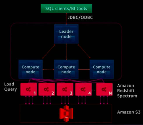
Amazon Redshift Spectrum architecture

The Load, unload, backup and restore of data is performed on Amazon S3. Amazon Redshift Spectrum is and extension of Amazon Redshift in which the nodes load data from Amazon S3 and execute queries directly against Amazon S3.

5.4.1.2. Terminology

5.4.1.2.1. Columnar

Amazon Redshift uses a columnar architecture for storing data on disk column by column rather than row by row like a traditional database. The reason for doing this is that the types of queries that you execute in an analytics database usually query a subset of the columns, so we are able to reduce the amount of IO needed to be done for analytics queries.

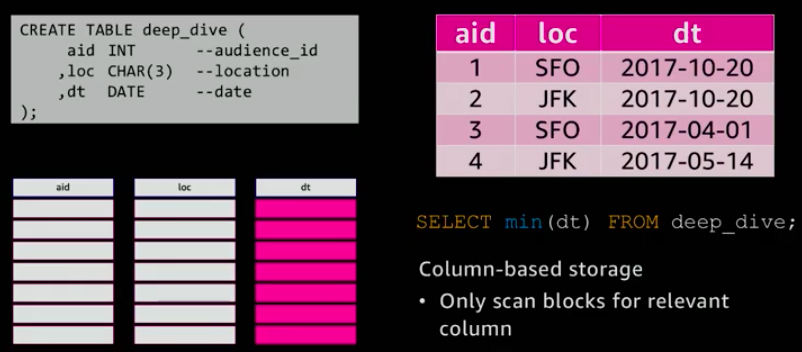
Columnar architecture: Example

In a columnar architecture, the data is stored physically on disk by column rather than by row. It only reads the column data that is required.

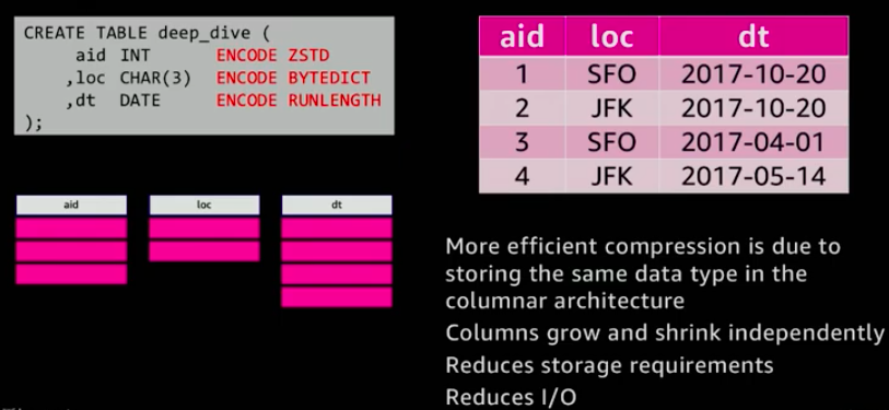
5.4.1.2.2. Compression

The goals of compression (sometimes called encoding) is to allow more data to be stored within an Amazon Redshift cluster and improve query performance by decreasing I/O. As a consequence, it allows several times more data to be stored within the cluster and also improves performance. The reason of this performance improvement is because it reduces the amount of I/O needed to do off disk.

By default, copy automatically analyzes and compresses data on first load into an empty table. The analyze compression is a built-in command that will find the optimal compression for each column on an existing table.

Compression: Example

The best practices are:

• To apply compression to all tables.
• Use analyze compression command to find the optimal compression. If it returns a encoding tyoe of RAW, it means that there is no compression, it happens for sparse columns and small tables.
• Changing column encoding requires a table rebuild: https://github.com/awslabs/amazon-redshift-utils/tree/master/src/ColumnEncodingUtility. To verify if columns are compressed:
• Verify that columns are compressed:

SELECT "column", type, encoding FROM pg_table_def WHERE tablename = 'deep_dive'

column |     type     | encoding
-------+--------------+----------
aid    | integer      | zstd
loc    | character(3) | bytedict
dt     | date         | runlength

5.4.1.2.3. Blocks

Column data is persisted to 1 MB immutable blocks. Blocks are individually encoded with 1 of 12 encodings. A full block con contain millions of values.

5.4.1.2.4. Zone maps

Zone maps are in-memory block metadata that contains per-block min and max values. All blocks automatically have zone maps. They effectively prunes blocks that cannot contain data for a given query. Their goal is to eliminate unnecessary I/O.

5.4.2. Data storage, ingestion, and ELT

5.4.3. Workload management and query monitoring

5.4.3.1. Workload management (WLM)

Workload management (WLM) allows for separation of different query workloads. Their main goals are prioritize important queries and throttle/abort less important queries. It allows us to control concurrent number of executing of queries, divide cluster memory and set query timeouts to abort long running queries.

Every single query in Redshift will execute in one queue. Queues are assigned a percentage of cluster memory. SQL queries execute in queue based on user group (which groups the user belongs to) and query group session level variable. WLM allows us to define the number of query queues that are available and how queries are routed to those queues for processing.

When you create a parameter group, the default WLM configuration contains one queue that can run up to five queries concurrently. You can add additional queues and configure WLM properties in each of them if you want more control over query processing. Each queue that you add has the same default WLM configuration until you configure its properties. When you add additional queues, the last queue in the configuration is the default queue. Unless a query is routed to another queue based on criteria in the WLM configuration, it is processed by the default queue. You cannot specify user groups or query groups for the default queue.

As with other parameters, you cannot modify the WLM configuration in the default parameter group. Clusters associated with the default parameter group always use the default WLM configuration. If you want to modify the WLM configuration, you must create a parameter group and then associate that parameter group with any clusters that require your custom WLM configuration.

Short query acceleration (SQA) allows to automatically detect short running queries and run them within the short query queue if queuing occurs.

5.4.3.2. Enhanced VPC Routing

When you use Amazon Redshift Enhanced VPC Routing, Amazon Redshift forces all COPY and UNLOAD traffic between your cluster and your data repositories through your Amazon VPC. By using Enhanced VPC Routing, you can use standard VPC features, such as VPC security groups, network access control lists (ACLs), VPC endpoints, VPC endpoint policies, internet gateways, and Domain Name System (DNS) servers. Hence, Option 2 is the correct answer.

You use these features to tightly manage the flow of data between your Amazon Redshift cluster and other resources. When you use Enhanced VPC Routing to route traffic through your VPC, you can also use VPC flow logs to monitor COPY and UNLOAD traffic. If Enhanced VPC Routing is not enabled, Amazon Redshift routes traffic through the Internet, including traffic to other services within the AWS network.

Configure enhanced VPC routing

5.4.4. Cluster sizing and resizing

5.4.5. Additional resources

You can configure Amazon Redshift to copy snapshots for a cluster to another region. To configure cross-region snapshot copy, you need to enable this copy feature for each cluster and configure where to copy snapshots and how long to keep copied automated snapshots in the destination region. When cross-region copy is enabled for a cluster, all new manual and automatic snapshots are copied to the specified region.

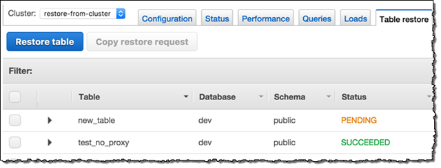
Restore table from snapshot on Redshift

AWS re:Invent 2018: [REPEAT 1] Deep Dive and Best Practices for Amazon Redshift (ANT401-R1)

5.4.6. Amazon Redshift Spectrum

Amazon Redshift also includes Redshift Spectrum, allowing you to directly run SQL queries against exabytes of unstructured data in Amazon S3. No loading or transformation is required, and you can use open data formats, including Avro, CSV, Grok, ORC, Parquet, RCFile, RegexSerDe, SequenceFile, TextFile, and TSV. Redshift Spectrum automatically scales query compute capacity based on the data being retrieved, so queries against Amazon S3 run fast, regardless of data set size.

5.5. Relational vs NoSQL databases

Relational databases vs NoSQL databases

Optimal workloads	They are designed for transactional and strongly consistent OLTP applications nad are good for OLAP.	NoSQL key-value, document, graph, and in-memory databases are designed for OLTP for a number of data access patterns that include low-latency applications. NoSQL, search databases are designed for analytics and semi-structured data.
Data model	The relational model normalizes data into tables that are composed of rows and columns. A schema strictly defines the tables, rows, columns, indexes, relationships between tables, and other database elements. The database enforces the referential integrity in relationships between tables.	NoSQL databases provide a variety of data models that includes document, graph, key-value, in-memory, and search.
ACID properties	They provide atomicity, consistency, isolation, and durability (ACID) properties: Atomicity requires a transaction to execute completely or not at all. Consistency requires that when a transaction has been committed, the data must conform to the database schema. Isolation requires that concurrent transactions execute separately for each other. Durability requires the ability to recover from an unexpected system failure or power outage to the last kown state.	They often make tradeoffs by relaxing some of the ACID properties of relational databases for a more flexible data model that can scale horizontally. This makes NoSQL databases an excellent choice for high throughput, low-latency use cases that need to scale horizontally beyond the limitations of a single instance.
Performance	Performance is generally dependent on the disk subsystem. The organization of the queries, indexes, and table structure is often required to achieve peak performance.	Performance is generally a function of the underlying HW cluster size, network latency, and the calling application.
Scale	They typically scale up by increasing the compute capabilities of the HW or scale-out by adding replicas for read-only workloads.	NoSQL databases typically are partitionable because key-value access patterns and able to scale out by using a distributed architecture to increase throughput that provides consistent performance at near boundless scale.
API	Requests to store and retrieve data are communicated using queries that conform to a structured query language (SQL). These queries are parsed and executed by the relational database.	Object-based APIs allow app developers to easily store and retrieve in-memory data structures. Partition keys let apps look up key-value pairs, column sets, or semistructured documents that contain serialized app objects and attributes.

5.6. Migrating data into your AWS databases

AWS Database Migration Service helps you migrate databases to AWS quickly and securely. The source database remains fully operational during the migration, minimizing downtime to applications that rely on the database. The AWS Database Migration Service can migrate your data to and from most widely used commercial and open-source databases.

AWS Database Migration Service can migrate your data to and from most of the widely used commercial and open source databases. It supports homogeneous migrations such as Oracle to Oracle, as well as heterogeneous migrations between different database platforms, such as Oracle to Amazon Aurora. Migrations can be from on-premises databases to Amazon RDS or Amazon EC2, databases running on EC2 to RDS, or vice versa, as well as from one RDS database to another RDS database. It can also move data between SQL, NoSQL, and text based targets.

In heterogeneous database migrations the source and target databases engines are different, like in the case of Oracle to Amazon Aurora, Oracle to PostgreSQL, or Microsoft SQL Server to MySQL migrations. In this case, the schema structure, data types, and database code of source and target databases can be quite different, requiring a schema and code transformation before the data migration starts. That makes heterogeneous migrations a two step process. First use the AWS Schema Conversion Tool to convert the source schema and code to match that of the target database, and then use the AWS Database Migration Service to migrate data from the source database to the target database. All the required data type conversions will automatically be done by the AWS Database Migration Service during the migration. The source database can be located in your own premises outside of AWS, running on an Amazon EC2 instance, or it can be an Amazon RDS database. The target can be a database in Amazon EC2 or Amazon RDS.